24. RNN Summary
Let's summarize what we have seen so far:
RNN Summary
As you have seen, in RNNs the current state depends on the input as well as the previous states, with the use of an activation function.
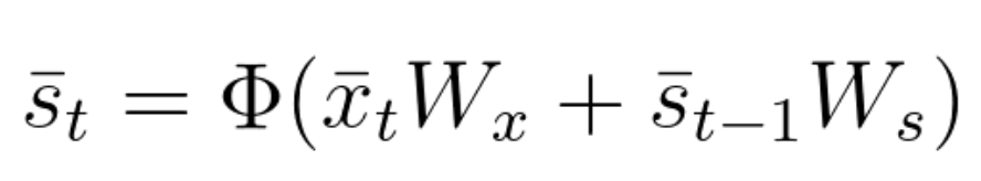
Equation 56
The current output is a simple linear combination of the current state elements with the corresponding weight matrix.
\bar{y}_t=\bar{s}_t W_y (without the use of an activation function)
or
\bar{y}_t=\sigma(\bar{s}_t W_y) (with the use of an activation function)
Equation 57
We can represent the recurrent network with the use of a folded model or an unfolded model:
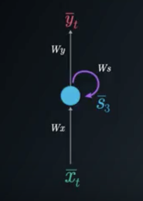
The RNN Folded Model
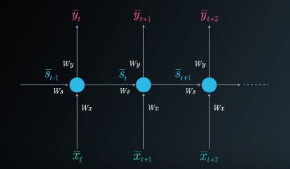
The RNN Unfolded Model
In the case of a single hidden (state) layer, we will have three weight matrices to consider. Here we use the following notations:
W_x - represents the weight matrix connecting the inputs to the state layer.
W_y - represents the weight matrix connecting the state to the output.
W_s - represents the weight matrix connecting the state from the previous timestep to the state in the following timestep.
The gradient calculations for the purpose of adjusting the weight matrices are the following:
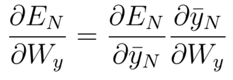
Equation 58
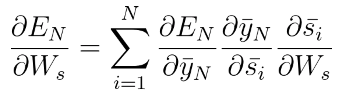
Equation 59
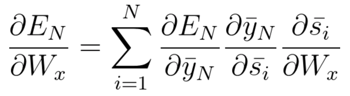
Equation 60
In equations 51 and 52 we used Backpropagation Through Time (BPTT) where we accumulate all of the contributions from previous timesteps.
When training RNNs using BPTT, we can choose to use mini-batches, where we update the weights in batches periodically (as opposed to once every inputs sample). We calculate the gradient for each step but do not update the weights right away. Instead, we update the weights once every fixed number of steps. This helps reduce the complexity of the training process and helps remove noise from the weight updates.
The following is the equation used for Mini-Batch Training Using Gradient Descent:
(where \delta_{ij} represents the gradient calculated once every inputs sample and M represents the number of gradients we accumulate in the process).
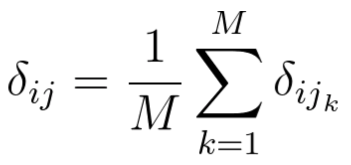
Equation 61
If we backpropagate more than ~10 timesteps, the gradient will become too small. This phenomena is known as the vanishing gradient problem where the contribution of information decays geometrically over time. Therefore temporal dependencies that span many time steps will effectively be discarded by the network. Long Short-Term Memory (LSTM) cells were designed to specifically solve this problem.
In RNNs we can also have the opposite problem, called the exploding gradient problem, in which the value of the gradient grows uncontrollably. A simple solution for the exploding gradient problem is Gradient Clipping.
More information about Gradient Clipping can be found here.
You can concentrate on Algorithm 1 which describes the gradient clipping idea in simplicity.